Simulating genetic drift
By Deependra Dhakal in R
November 8, 2020
Genetic drift is the result of bernouli process on survival of individuals (given some probability for each of them) of a population over a number of independent trials (Generation).
Apparently there are two techniques of seeing such process – one individual level, other the population level. Both solutions are illustrated below. Let us suppose population of N individuals remains fixed from generation to generation, likewise, Fitness probability of “A” allele ($p(A)$) and “a” allele ($p(a)$) both starts off equal. Now we can generate incremental population survival probability for each individual for given population size:
N <- 100
pA <- vector()
pA[1] <- 0.5
i <- 1

while ((pA[i] < 1) & (pA[i] > 0)) {
  nA <- 0

  for (j in 1:N){
    random <- runif(1)
    if(random < pA[i]){nA <- nA + 1}
  }
  pA[i + 1] <- nA/N
  i <- i + 1
}
Alternatively rbinom function generates the same but with probabilistic draw from entire population.
drift_generate <- function(N = 100){
N <- N
pA <- vector()
pA[1] <- 0.5
i <- 1
while ((pA[i] < 1) & (pA[i] > 0)) {
nA <- rbinom(n = 1, size = N, prob = pA[i])
pA[i + 1] <- nA/N
i <- i + 1
}
return(tidyr::tibble(i = 1:i, pA = pA))
}
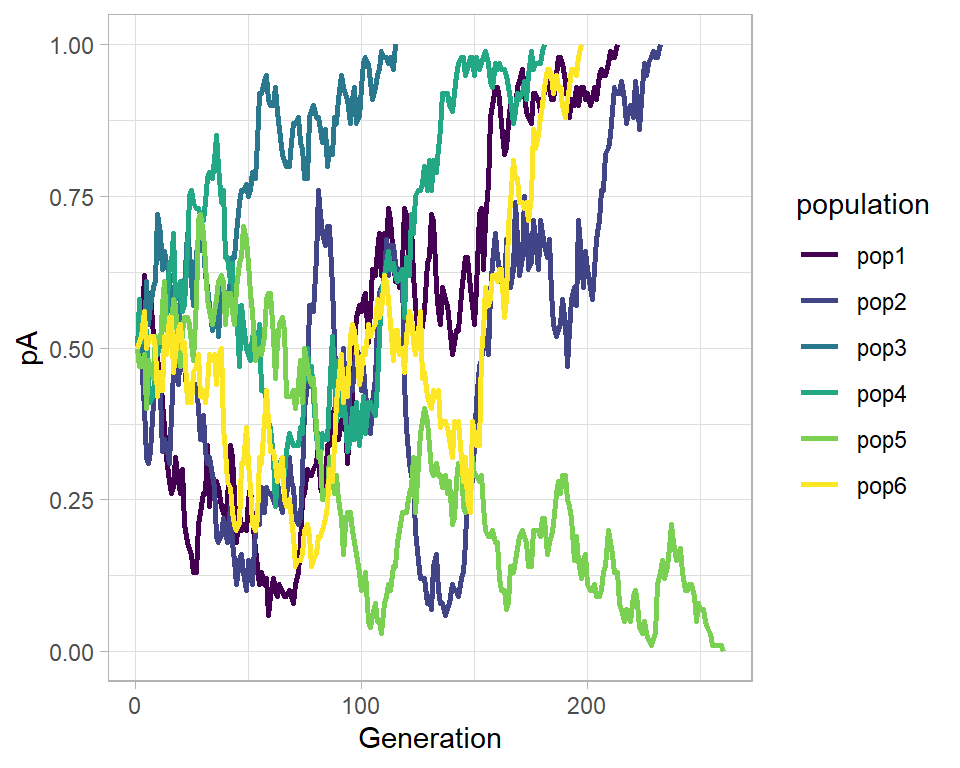
drift_tibble <- purrr::map_dfr(c(pop1 = 1, pop2 = 2,
pop3 = 3, pop4 = 4,
pop5 = 5, pop6 = 6),
~drift_generate(N = 100), .id = "population")
drift_gg <- ggplot(aes(x = i, y = pA), data = drift_tibble) +
# geom_point(aes(color = population)) +
geom_path(aes(color = population), size = 1.0) +
theme_light() +
scale_color_viridis_d() +
labs(x = "Generation")
drift_gg
- Posted on:
- November 8, 2020
- Length:
- 2 minute read, 270 words
- Categories:
- R
- Tags:
- population genetics R