Dealing with factors

By Deependra Dhakal in R factor blog

May 18, 2017

A `factor` is an headache

I have a dataset, cleaning which has been a pain lately. I’m going to use 20 observations of the imported dataset in this post to demonstrate how pathetically have I been advancing with it.

plot	jan_23_2017	jan_26_2017	jan_29_2017	feb_02_2017
1	0	0	b	am
2	f	s	1p	10p
3	b	a	sm	3p
4	b	b	ap	2
5	0	b	bp	s
6	b	a	sp	3

Providing it a context, the columns represent multiple observations of same variable at different dates, as apparent from the column names.

One can observe from the str(head_boot) that the dataframe has only 20 observations. Had a larger dataframe been subsetted, the factors with their usual nuisance carry over the all the levels, even currently unused ones. To demonstrate this, below I present how many factor levels the original dataframe had and what changes after a subset (slice, filter have same feature) operation.

# original dataframe
head_boot %>% 
  select_if(is.factor) %>% 
  map_int(function(x)length(levels(x)))

## jan_23_2017 jan_26_2017 jan_29_2017 feb_02_2017 
##           5           6          14          15

# subsetted to obtain a dataframe where one factors has either "s" or "0" levels only
subset.data.frame(head_boot, 
                  subset = head_boot$jan_23_2017 %in% c("s", "0"), 
                  select = sapply(head_boot, is.factor)) %>% 
  map_int(function(x)length(levels(x)))

## jan_23_2017 jan_26_2017 jan_29_2017 feb_02_2017 
##           5           6          14          15

All factor levels are retained !

A prophylactic measure is avoiding at all importing of character data columns as a factor. This could be done using setup option: options(stringsAsFactors = FALSE) ahead of import. Still, after the import many options exist. Some of the best alternatives out are listed below:

Use subsetted_df$factor_col[, drop=TRUE], where a vector of factor values is indexed with drop argument.
Convert factor columns of subsetted dataframe first to character and then back to factors class.
Use forcats::fct_drop(f) for more reliable NA handling
Use droplevels() or droplevels.data.frame()

To give a realistic feel to data, factor levels may be recoded or relabelled with more informative labels.

suit_labels <- factor(c("before_boot_n_boot", "heading", "anthesis"), 
                      levels = c("before_boot_n_boot", "heading", "anthesis"), 
                      ordered = T)

# what are all the levels
head_boot_lvl <- head_boot %>% 
  select_if(is.factor) %>% 
  map(levels) %>% 
  unlist() %>% 
  unique()

# create all combinations of factor levels of the dataset
# purrr::cross_df preserves the order, tidyr::crossing doesn't
possible_hb_lvl <- cross_df(list(post  = factor(c("m", "", "p"), ordered = TRUE), 
      pre = factor(c("b", "f", "a", "s", "1", "2", 
                     "3", "4", "10", "11", "12"), ordered = TRUE))) %>% 
  select(rev(everything())) %>% 
  # arrange(match(post, c("m", "", "p"))) %>% # don't need this ordering 
  unite(col = "pre_post", sep = "") %>% 
  add_row(pre_post = "0", .before = 1) %>% 
  mutate(pre_post = factor(pre_post, levels = pre_post, ordered = TRUE))

# mutate original dataframe to represent ordinal factors
head_boot <- head_boot %>% 
  mutate_if(is.factor, function(x)factor(x, levels = possible_hb_lvl$pre_post, labels = possible_hb_lvl$pre_post, ordered = TRUE))

# function to recode factor levels (better to use `fct_recode()`)
fct_minimize <- function(x)case_when(x < "1m" ~ suit_labels[1], 
                                     x >= "1m" & x < "10m" ~ suit_labels[2], 
                                     x >= "10m" ~ suit_labels[3], 
                                     TRUE ~ NA)

# mutate original dataframe with function to recode factor levels
head_boot <- head_boot %>% 
  mutate_if(is.factor, fct_minimize)

str(head_boot)

## tibble [20 × 5] (S3: tbl_df/tbl/data.frame)
##  $ plot       : num [1:20] 1 2 3 4 5 6 7 8 9 10 ...
##  $ jan_23_2017: Ord.factor w/ 3 levels "before_boot_n_boot"<..: 1 1 1 1 1 1 1 1 1 1 ...
##  $ jan_26_2017: Ord.factor w/ 3 levels "before_boot_n_boot"<..: 1 1 1 1 1 1 1 2 1 1 ...
##  $ jan_29_2017: Ord.factor w/ 3 levels "before_boot_n_boot"<..: 1 2 1 1 1 1 2 2 2 1 ...
##  $ feb_02_2017: Ord.factor w/ 3 levels "before_boot_n_boot"<..: 1 3 2 2 1 2 2 3 2 1 ...

A more telling dataframe looks like the one below.

knitr::kable(head(head_boot), format = "html", align = "c") %>% 
  kableExtra::kable_styling(bootstrap_options = c("striped", "hover"), 
                            font_size = 10, position = "center") %>% 
  kableExtra::row_spec(0, bold = TRUE) %>% 
  kableExtra::column_spec(1, bold = TRUE)

plot	jan_23_2017	jan_26_2017	jan_29_2017	feb_02_2017
1	before_boot_n_boot	before_boot_n_boot	before_boot_n_boot	before_boot_n_boot
2	before_boot_n_boot	before_boot_n_boot	heading	anthesis
3	before_boot_n_boot	before_boot_n_boot	before_boot_n_boot	heading
4	before_boot_n_boot	before_boot_n_boot	before_boot_n_boot	heading
5	before_boot_n_boot	before_boot_n_boot	before_boot_n_boot	before_boot_n_boot
6	before_boot_n_boot	before_boot_n_boot	before_boot_n_boot	heading

Visualizing data

Bar plotting of the ordinal data might reveal interesting insights, so let’s prepare ggplot graphs.

walk2(.x = head_boot %>% select(jan_23_2017:feb_02_2017) %>% colnames(),
      .y = as.character(strptime(str_subset(colnames(head_boot), "^\\w{3}_\\d{2}"), 
                                 format = "%b_%d_%Y")),
      .f = ~print(ggplot(aes(x = get(.x)), data = head_boot) +
                    geom_bar(position = "dodge", stat = "count", width = .5) +
                    xlab(.y) +
                    theme(axis.text.x = element_text(angle = 40, size = 9, vjust = 0.6))))

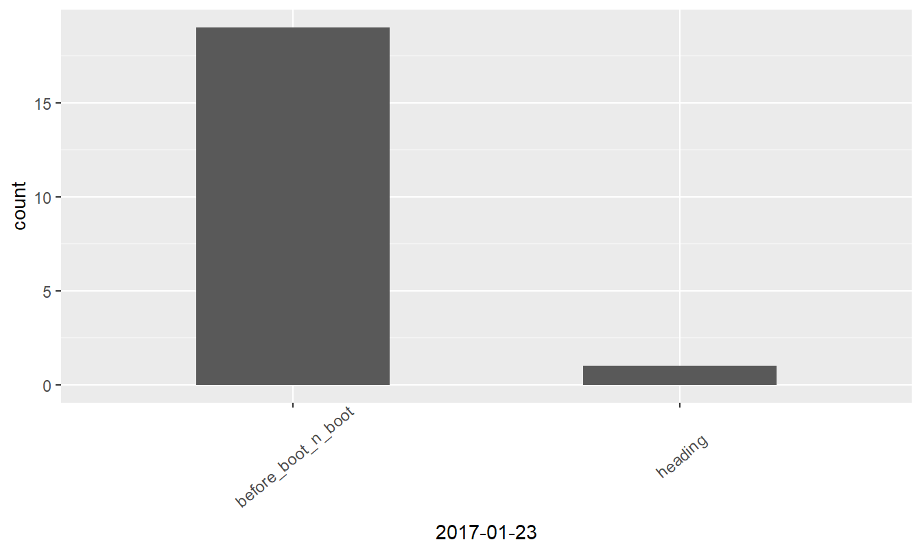
Figure 1: Growth stages at different dates

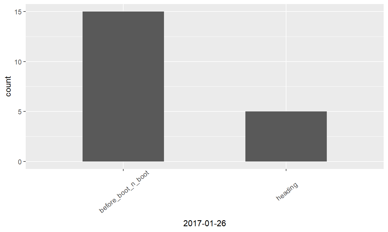
Figure 2: Growth stages at different dates

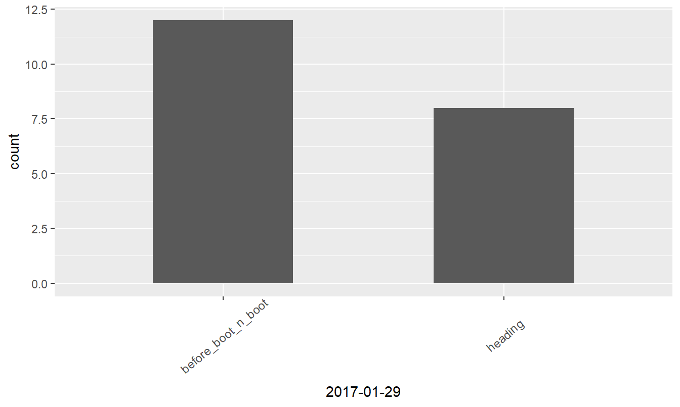
Figure 3: Growth stages at different dates

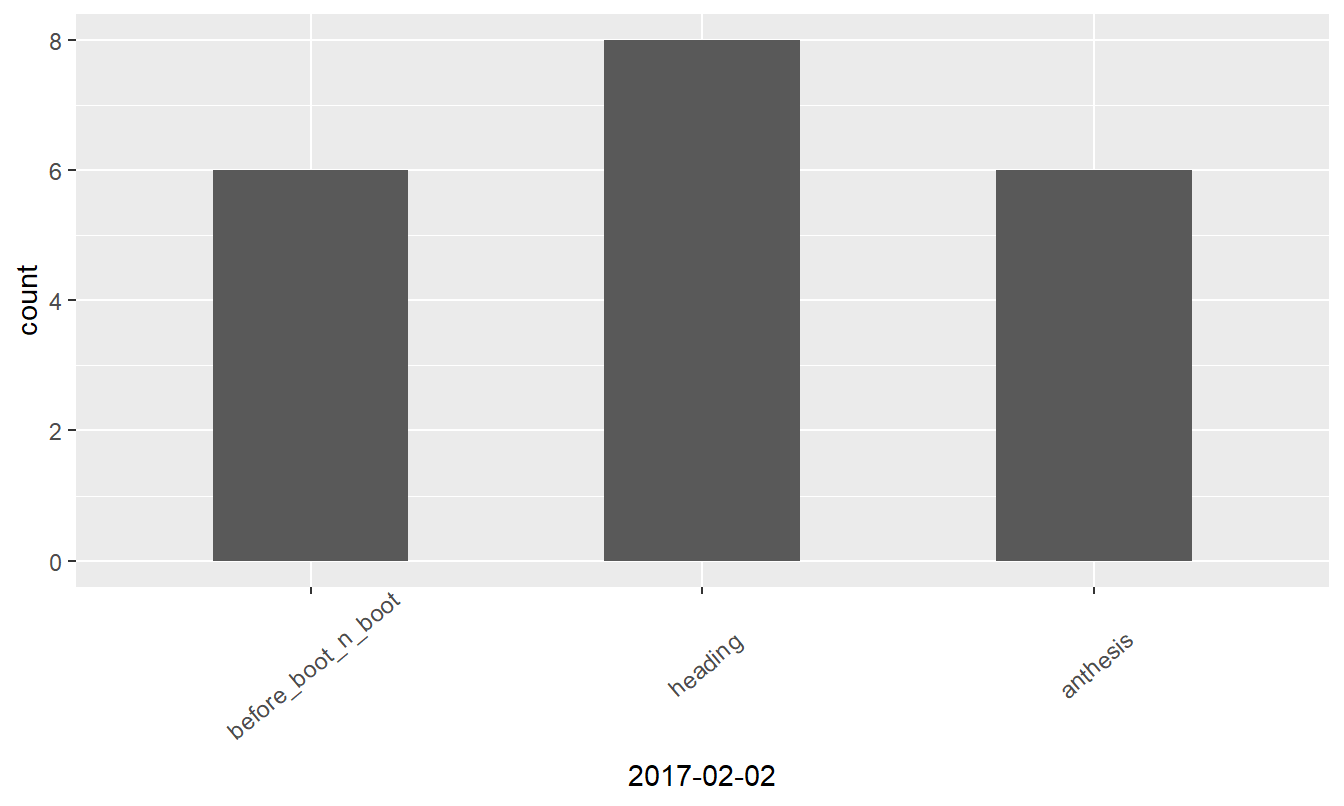
Figure 4: Growth stages at different dates

With dplyr, It’s seemless to obtain a tabular summary of what has been visualized above.

# credit: https://stackoverflow.com/a/46340237/6725057
head_boot %>% 
  select_if(is.factor) %>% 
  tidyr::gather(date, stage) %>% 
  dplyr::group_by(date, stage) %>% 
  dplyr::count() %>% 
  dplyr::ungroup() %>% 
  tidyr::spread(date, n) %>% 
  knitr::kable(format = "html", align = "c") %>% 
  kableExtra::kable_styling(bootstrap_options = c("striped", "hover"), 
                            font_size = 10, position = "center") %>% 
  kableExtra::row_spec(0, bold = TRUE) %>% 
  kableExtra::column_spec(1, bold = TRUE)

stage	feb_02_2017	jan_23_2017	jan_26_2017	jan_29_2017
anthesis	6
before_boot_n_boot	6	19	15	12
heading	8	1	5	8

Posted on:: May 18, 2017

Length:: 4 minute read, 847 words

Categories:: R factor blog

Tags:: R factors

See Also:: Simulating genetic drift; Missing negative from the normal; Internals of Mixed Models

A factor is an headache

Visualizing data

A `factor` is an headache