Linear model fitting for regression: Basics and Variation

Linear model (simple forms) fitting

I use mtcars dataset to construct some basic regression models and fit those.

# convert available data to use in fitting
mtcars_reg_df <- mtcars %>% 
  rownames_to_column("carnames") %>% 
  as_tibble() %>% 
  mutate_at(c("gear", "am", "vs", "cyl"), as.factor)

We will be comparing difference between cylinder means for mpg.

# # intercept only lm tidiying and visualization
mpg_model1 <- mtcars_reg_df %>%
  group_by(cyl) %>%
  nest() %>%
  group_by(cyl) %>%
  mutate(mpg_model = map(data, ~lm(`mpg` ~ 1, .x))) %>%
  mutate(
    # rsqrd = map_dbl(mpg_model, ~summary(.x)[['r.squared']]), # this is '0' of intercept only model
    intercept_pvalue = map_dbl(mpg_model, ~summary(.x)[['coefficients']][1, 4]),
    intercept_se = map_dbl(mpg_model, ~summary(.x)[['coefficients']][1, 2]),
    intercept_coef = map_dbl(mpg_model, ~summary(.x)[['coefficients']][1, 1])
  ) %>%
  select(cyl, mpg_model, contains("intercept"), data)

Intercept-only models (each group fitted a different one) are plotted to reflect variation in estimated parameters. Two methods can be used to obtain same result. In the first, standard error obtained from model summary can be directly used; in the other SE can be manually computed.
By Deependra Dhakal

August 7, 2020

Disease epidemiology: A simulation scenario of infectious viral disease (COVID-19)

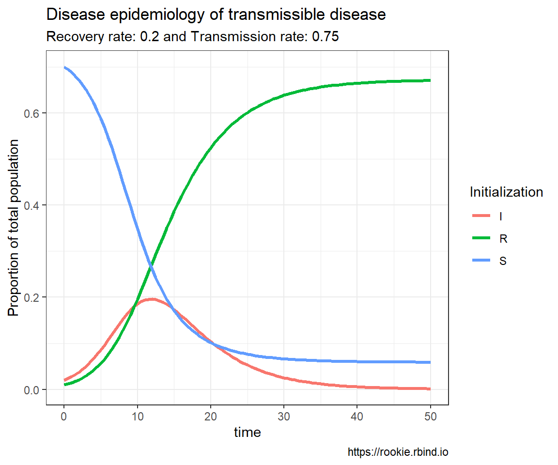
SIR model of COVID-19 epidemiology

## # A tibble: 5,555 × 6
##    beta_id  time       S      I      R beta_value
##    <chr>   <dbl>   <dbl>  <dbl>  <dbl>      <dbl>
##  1 1         0   0.7     0.02   0.01          3.2
##  2 1         0.5 0.662   0.0541 0.0134        3.2
##  3 1         1   0.575   0.133  0.0223        3.2
##  4 1         1.5 0.420   0.268  0.0420        3.2
##  5 1         2   0.242   0.411  0.0763        3.2
##  6 1         2.5 0.117   0.491  0.122         3.2
##  7 1         3   0.0521  0.506  0.172         3.2
##  8 1         3.5 0.0235  0.484  0.222         3.2
##  9 1         4   0.0111  0.450  0.269         3.2
## 10 1         4.5 0.00559 0.413  0.312         3.2
## # ℹ 5,545 more rows

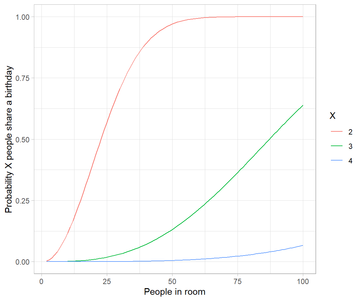
The birthday problem: Non analytical solution

# Birthday problem

crossing(n = 2:100, 
         x = 2:4) %>% 
  mutate(probability = map2_dbl(n, x, ~pbirthday(.x, coincident = .y))) %>% 
  ggplot(aes(n, probability, color = factor(x))) +
  geom_line() +
  labs(x = "People in room", 
       y = "Probability X people share a birthday", 
       color = "X")
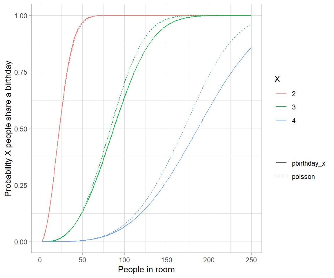
# Approximating birthday paradox with Poisson distribution

crossing(n = 2:250, 
         x = 2:4) %>% 
  mutate(combinations = choose(n, x), 
         probability_each = (1/365)^(x-1), 
         poisson = 1-dpois(0, combinations * probability_each), 
         pbirthday_x = map2_dbl(n, x, ~pbirthday(.x, coincident = .y))) %>% 
  gather(type, probability, pbirthday_x, poisson) %>% 
  ggplot(aes(n, probability, color = factor(x), lty = type)) +
  geom_line() +
  labs(x = "People in room", 
       y = "Probability X people share a birthday", 
       color = "X", 
       lty = "")
# the reason is because events are no longer weakly dependent-every pair makes triplets
# more likely.

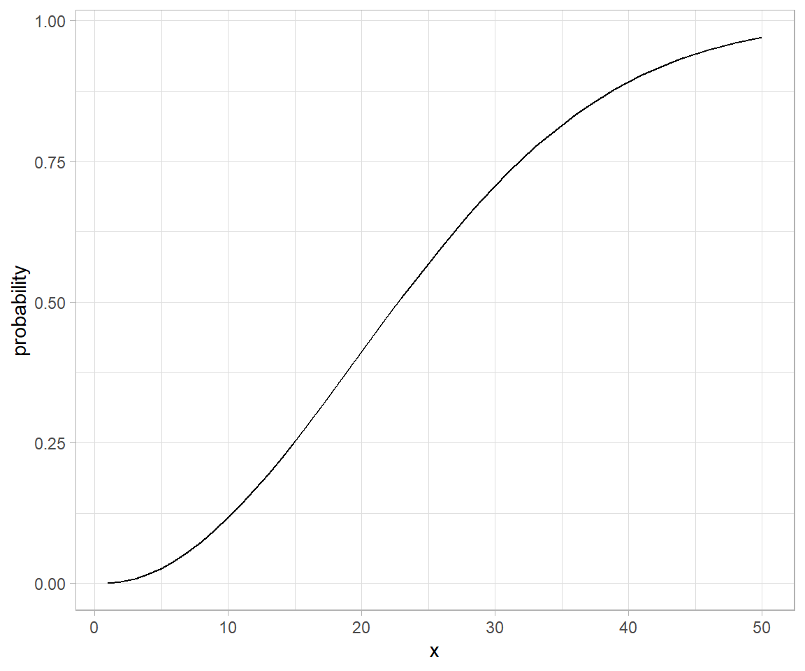
# Analytical solution to birthday problem (Mikhail Papov; bearlogic.github.io)

# Suppose, we are interested in the probability that, in a set of n randomly chosen people, some pair of them will have the same
# birthday (which we refer to as event A).

# Using Kolmogorov axionms and conditional probability, we can derive an analytical solution for P(A):

# P(A) = 1-\frac{n!.\binom{365}{n}}{365^n}

# This can be solved in `R` as:

pa <- function(n){
  1 - (factorial(n) * choose(365, n))/(365^n)
}

map_dfr(.x = list(probability = 1:50), .f = pa) %>% 
  mutate(x = seq_along(probability)) %>% 
  ggplot(aes(x = x, y = probability)) +
  geom_line()

By Deependra Dhakal in R

August 6, 2020

Piecewise Linear Function: An Introduction

Definition and meaning

Wikipedia defines a piecewise linear function as:

“a function defined on a (possibly unbounded) interval of real numbers, such that there is a collection of intervals on each of which the function is an affine function”

Example

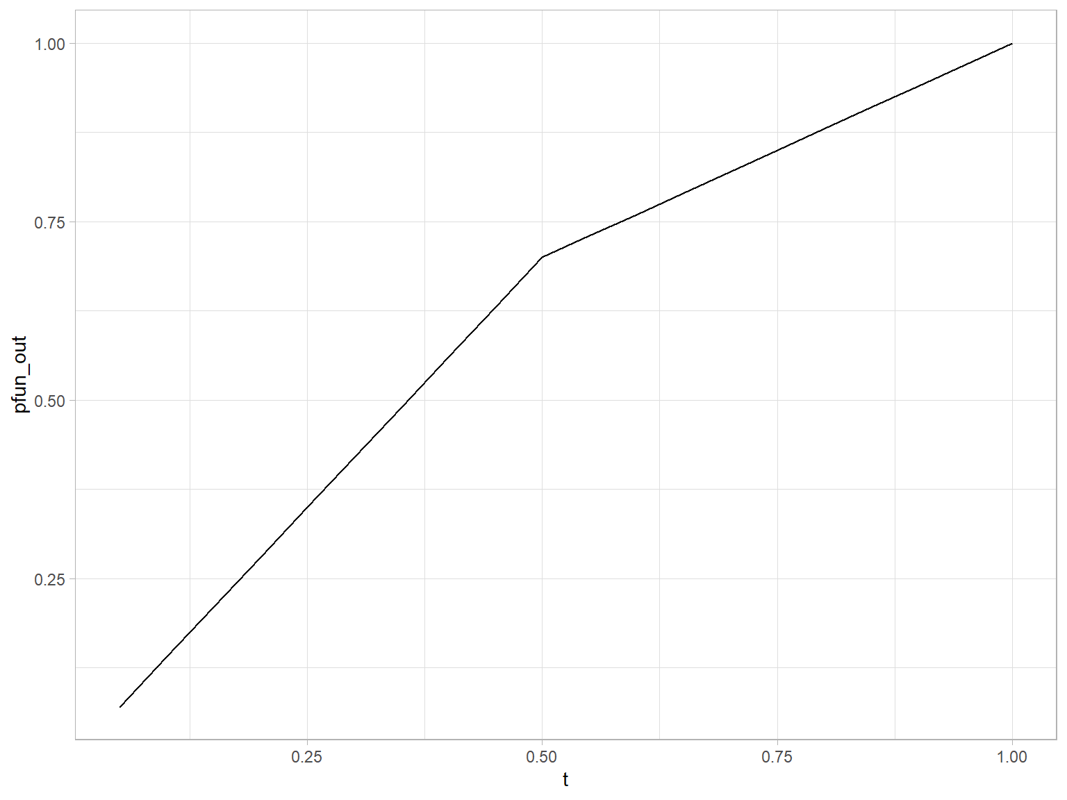
# piecewise linear functions using if statements

# piecewise linear function defined using if for cases.
pw.function <- function(t) {
  if(t < 0.5) {
    0.7 * t/0.5
  } else {
    0.7 + 0.3*(t-0.5)/0.5
  }
}

pw.function <- Vectorize(pw.function)

tibble(t = seq(0.05:0.99, by = 0.05)) %>% 
  mutate(pfun_out = pw.function(t)) %>%
  ggplot() +
  geom_line(aes(x = t, y = pfun_out), group = "combined_grp")

Application

In segmentation and curve fitting. For a larger discourse refer to segmented package in cran.

By Deependra Dhakal in R

August 6, 2020