Tidyverse

Cluster dendrogram: An introduction and showcase

A cluster analysis is a classification problem. It is dealt in several ways, one of which is hierarchial agglomeration. The method allows for easy presentation of high dimensional data, more of so when the number of observations is readily fitted into a visualization.

Here’s I deal with a case of clustering typically seen in agriculture and field research where a researcher tests typically a large number of genotypes and seeks to see them organized into distinguishable clusters using dendrogram. Data concerns observations on disease incidence in rice genotypes of various stages – germinating seed to maturity nearing crop. Following provides a descriptive summary of the observation variables.
Logistic Regression: Part II - Varietal adoption dataset

Binary classifier using categorical predictor

Let’s say we have two variable – survey response of farmer to willingness to adopt improved rice variety (in YES/NO) and them having been trained earlier about agricultural input management (in trained/untrained).

Read in the data and notice the summary.

rice_data <- readxl::read_xlsx(here::here("content", "blog", "data", "rice_variety_adoption.xlsx")) %>% 
  mutate_if(.predicate = is.character, as.factor)

rice_variety_adoption <- readxl::read_xlsx(here::here("content", "blog", "data", "rice_variety_adoption.xlsx")) %>%
  select(improved_variety_adoption, training) %>% 
  # convert data to suitable factor type for analysis.
  mutate_if(is.character, as.factor)

head(rice_variety_adoption) # now we have data
## # A tibble: 6 × 2
##   improved_variety_adoption training
##   <fct>                     <fct>   
## 1 No                        No      
## 2 Yes                       No      
## 3 No                        No      
## 4 Yes                       No      
## 5 Yes                       No      
## 6 No                        No

As a basic descriptive, contruct one way and two way cross tabulation summary, showing count of each categories. This is because logistic regression uses count data, much like in a non-parametric model.

Logistic Regression: Part I - Fundamentals

Likelihood theory

Probit models were the first of those being used to analyze non-normal data using non-linear models. In an early example of probit regression, Bliss(1934) describes an experiment in which nicotine is applied to aphids and the proportion killed is recorded. As an appendix to a paper Bliss wrote a year later (Bliss, 1935), Fisher (1935) outlines the use of maximum likelihood to obtain estimates of the probit model.

Linear model fitting for regression: Basics and Variation

Linear model (simple forms) fitting

I use mtcars dataset to construct some basic regression models and fit those.

# convert available data to use in fitting
mtcars_reg_df <- mtcars %>% 
  rownames_to_column("carnames") %>% 
  as_tibble() %>% 
  mutate_at(c("gear", "am", "vs", "cyl"), as.factor)

We will be comparing difference between cylinder means for mpg.

# # intercept only lm tidiying and visualization
mpg_model1 <- mtcars_reg_df %>%
  group_by(cyl) %>%
  nest() %>%
  group_by(cyl) %>%
  mutate(mpg_model = map(data, ~lm(`mpg` ~ 1, .x))) %>%
  mutate(
    # rsqrd = map_dbl(mpg_model, ~summary(.x)[['r.squared']]), # this is '0' of intercept only model
    intercept_pvalue = map_dbl(mpg_model, ~summary(.x)[['coefficients']][1, 4]),
    intercept_se = map_dbl(mpg_model, ~summary(.x)[['coefficients']][1, 2]),
    intercept_coef = map_dbl(mpg_model, ~summary(.x)[['coefficients']][1, 1])
  ) %>%
  select(cyl, mpg_model, contains("intercept"), data)

Intercept-only models (each group fitted a different one) are plotted to reflect variation in estimated parameters. Two methods can be used to obtain same result. In the first, standard error obtained from model summary can be directly used; in the other SE can be manually computed.

The birthday problem: Non analytical solution

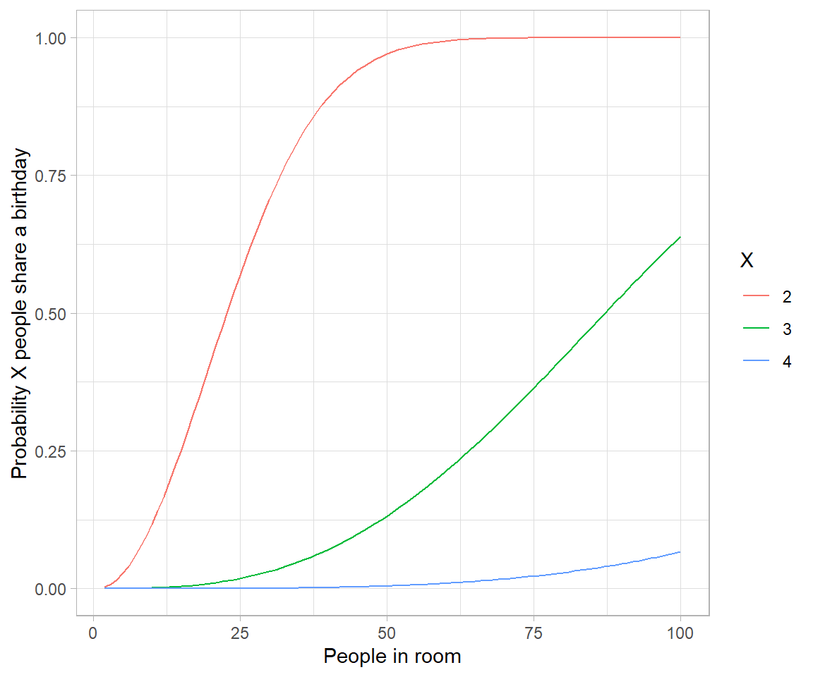
# Birthday problem

crossing(n = 2:100, 
         x = 2:4) %>% 
  mutate(probability = map2_dbl(n, x, ~pbirthday(.x, coincident = .y))) %>% 
  ggplot(aes(n, probability, color = factor(x))) +
  geom_line() +
  labs(x = "People in room", 
       y = "Probability X people share a birthday", 
       color = "X")
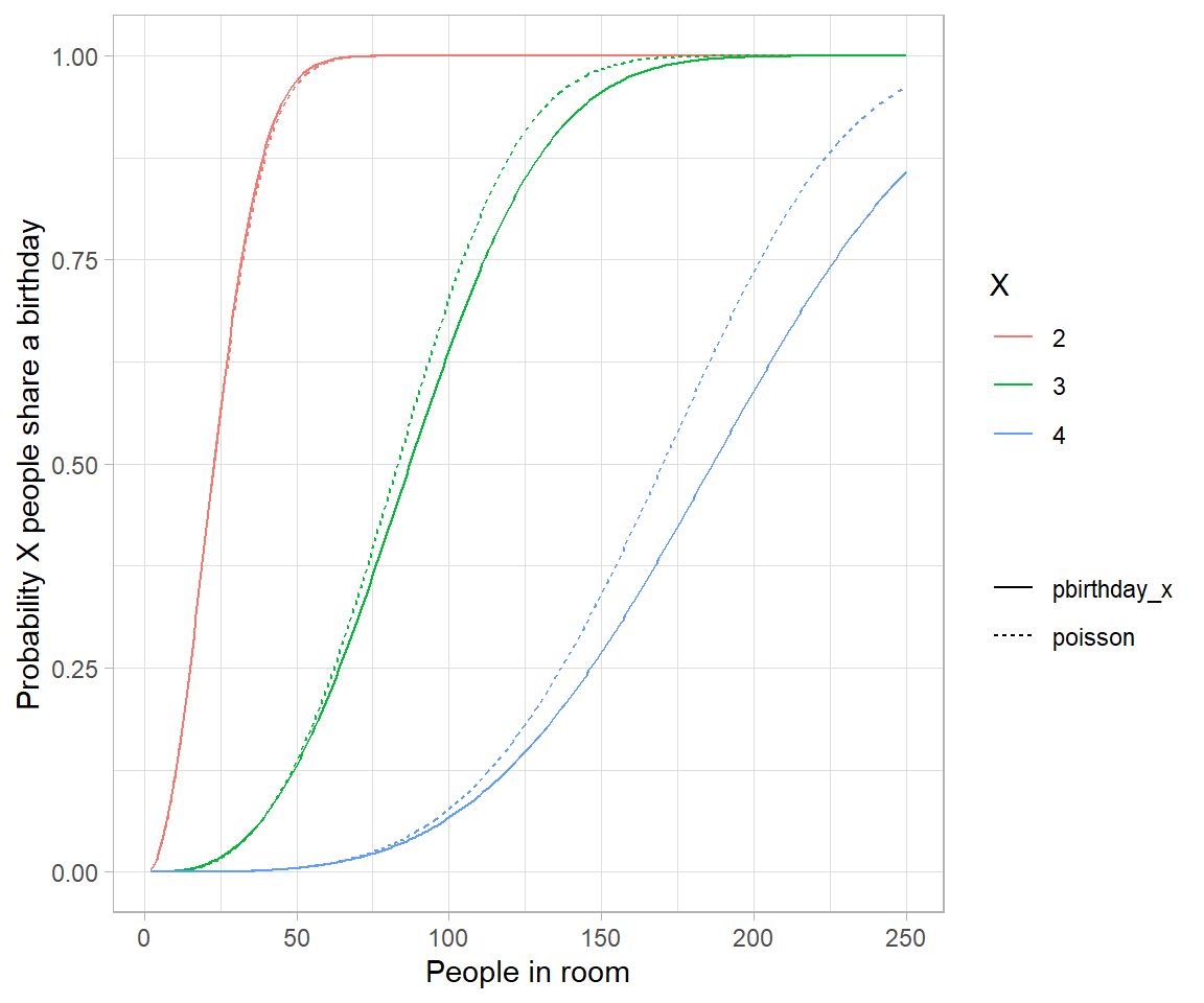
# Approximating birthday paradox with Poisson distribution

crossing(n = 2:250, 
         x = 2:4) %>% 
  mutate(combinations = choose(n, x), 
         probability_each = (1/365)^(x-1), 
         poisson = 1-dpois(0, combinations * probability_each), 
         pbirthday_x = map2_dbl(n, x, ~pbirthday(.x, coincident = .y))) %>% 
  gather(type, probability, pbirthday_x, poisson) %>% 
  ggplot(aes(n, probability, color = factor(x), lty = type)) +
  geom_line() +
  labs(x = "People in room", 
       y = "Probability X people share a birthday", 
       color = "X", 
       lty = "")
# the reason is because events are no longer weakly dependent-every pair makes triplets
# more likely.

# Analytical solution to birthday problem (Mikhail Papov; bearlogic.github.io)

# Suppose, we are interested in the probability that, in a set of n randomly chosen people, some pair of them will have the same
# birthday (which we refer to as event A).

# Using Kolmogorov axionms and conditional probability, we can derive an analytical solution for P(A):

# P(A) = 1-\frac{n!.\binom{365}{n}}{365^n}

# This can be solved in `R` as:

pa <- function(n){
  1 - (factorial(n) * choose(365, n))/(365^n)
}

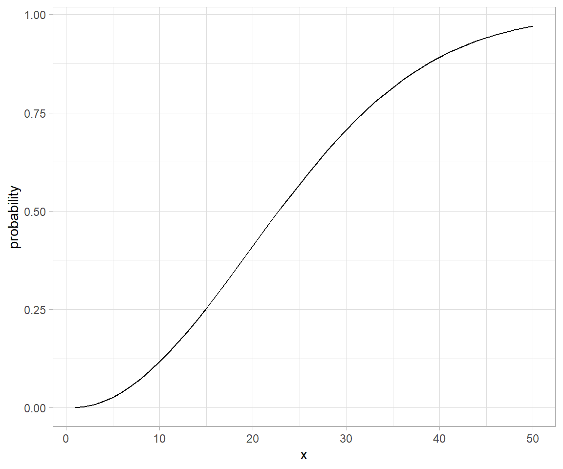
map_dfr(.x = list(probability = 1:50), .f = pa) %>% 
  mutate(x = seq_along(probability)) %>% 
  ggplot(aes(x = x, y = probability)) +
  geom_line()

Piecewise Linear Function: An Introduction

Definition and meaning

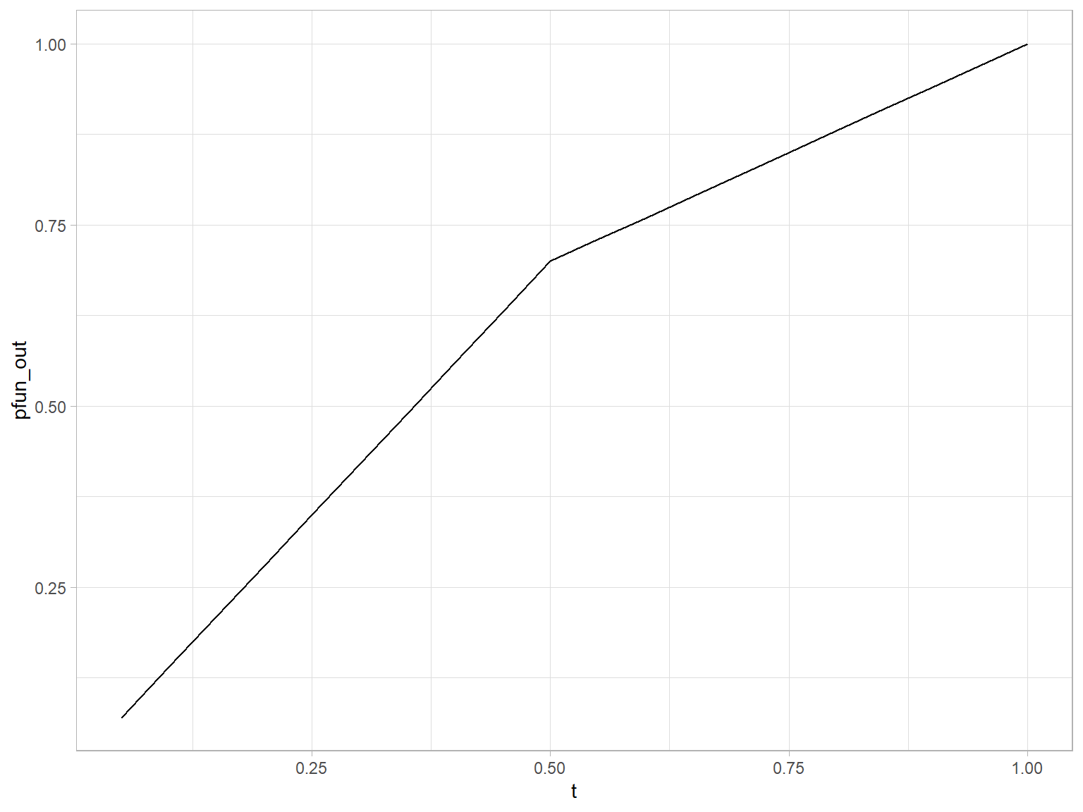
Wikipedia defines a piecewise linear function as:

“a function defined on a (possibly unbounded) interval of real numbers, such that there is a collection of intervals on each of which the function is an affine function”

Example

# piecewise linear functions using if statements

# piecewise linear function defined using if for cases.
pw.function <- function(t) {
  if(t < 0.5) {
    0.7 * t/0.5
  } else {
    0.7 + 0.3*(t-0.5)/0.5
  }
}

pw.function <- Vectorize(pw.function)

tibble(t = seq(0.05:0.99, by = 0.05)) %>% 
  mutate(pfun_out = pw.function(t)) %>%
  ggplot() +
  geom_line(aes(x = t, y = pfun_out), group = "combined_grp")

Application

In segmentation and curve fitting. For a larger discourse refer to segmented package in cran.

String tip: complex pattern recognition

Background

This post is all about examples and use cases. So…Let’s break a leg.

  1. Extract all words except last one using anchors and look arounds
nasty_char <- c("I love playing wildly") # remove the last word "wildly"

stringr::str_extract(nasty_char, ".*(?=\\s[:alpha:]*$)")
## [1] "I love playing"

Expressing timestamp data in calendar

Unlike composing a text memos and keeping tracks of those, calendar graphics is a highly effective visual aid to taking notes and summarizing them. Well, we all have used calendar, one way or the other, in our lifetimes.

Calendar based graphics enables an accurate catch at the very first glance; For example, it is very easy relating one activity of a period to another when they are laid linearly with precise graduations. Calendar graphics does exactly that – some features (usually tiles) provide graduation, representing fixed interval of time (e.g., a day). This when combined with text allows unlimited freedom to provide narration for specific intervals.

Grade X result


Total Marks and Final Grades {-}

roll number English Total Marks Nepali Total Marks C. Maths Total Marks Science Total Marks Extension Total Marks Soil Total Marks Plant protection Total Marks Fruit Total Marks Agronomy Total Marks Computer Total Marks O. Maths Total Marks English Total Marks Agg grade Nepali Total Marks Agg grade C. Maths Total Marks Agg grade Science Total Marks Agg grade Extension Total Marks Agg grade Soil Total Marks Agg grade Plant protection Total Marks Agg grade Fruit Total Marks Agg grade Agronomy Total Marks Agg grade Computer Total Marks Agg grade O. Maths Total Marks Agg grade
1 70.2 57.2 NA 72.4 77.3 84.9 81.9 74.8 88.2 88.3 NA B+ C+ NA B+ B+ A A B+ A A NA
2 76.8 46.2 NA 63.2 72.1 82 77 71.7 81.2 74.7 NA B+ C NA B B+ A B+ B+ A B+ NA
3 82.8 57 NA 56 89.8 82.5 82.1 85.3 89.7 79 NA A C+ NA C+ A A A A A B+ NA
4 42.4 19.5 NA 20.6 48.8 58.2 50.1 49.8 54.8 67 NA C E NA D C C+ C+ C C+ B NA
5 55.2 34.3 NA 33.2 49.6 64.2 59.8 57.1 61 73.3 NA C+ D NA D C B C+ C+ B B+ NA
6 49.5 43.3 NA 24.8 51.7 55.5 52.9 46.4 55.4 65.5 NA C C NA D C+ C+ C+ C C+ B NA
7 71.4 50.4 NA 54.8 75.7 71.6 76.8 61.7 80.6 77.2 NA B+ C+ NA C+ B+ B+ B+ B A B+ NA
8 73.8 45.3 NA 62 83.9 81.7 78.1 83.6 88.2 79.4 NA B+ C NA B A A B+ A A B+ NA
9 51.9 39.9 NA 26.8 56.9 56 62 49.6 57.2 64.7 NA C+ D NA D C+ C+ B C C+ B NA
10 NA NA NA NA NA NA NA NA NA NA NA NA NA NA NA NA NA NA NA NA NA NA
11 42 20.6 NA 22.1 49.2 54.2 53.8 44.5 51.2 59.3 NA C D NA D C C+ C+ C C+ C+ NA
12 52.6 22 NA 36.9 57.9 69.6 67.1 61.2 65.8 68.2 NA C+ D NA D C+ B B B B B NA
13 61.8 30.8 NA 27.9 59.5 65.8 63.3 53.8 62.4 70.7 NA B D NA D C+ B B C+ B B+ NA
14 58.8 32.6 NA 19 51.8 54.7 63.3 48.4 60.1 68 NA C+ D NA E C+ C+ B C B B NA
15 69.3 34.6 NA 35.1 55.3 62.3 63.5 63.8 66.2 80.6 NA B D NA D C+ B B B B A NA
16 54.9 23.9 NA 29 48.7 56.6 54.4 53.4 55.7 59.6 NA C+ D NA D C C+ C+ C+ C+ C+ NA
17 58.2 37.2 NA 25.7 66.9 66.6 66.3 62.8 70.1 64.4 NA C+ D NA D B B B B B+ B NA
18 NA NA NA NA NA NA NA NA NA NA NA NA NA NA NA NA NA NA NA NA NA NA
19 48.7 40.9 NA 27.4 77.1 72.8 70 66.5 75.2 62.6 NA C C NA D B+ B+ B+ B B+ B NA
20 48.1 26.5 NA 22.9 56.7 64.6 54 51.2 64.6 61.9 NA C D NA D C+ B C+ C+ B B NA
21 NA NA NA NA NA NA NA NA NA NA NA NA NA NA NA NA NA NA NA NA NA NA
22 70.5 42.8 NA 55 70.5 74.4 60.8 73.2 81.5 73.2 NA B+ C NA C+ B+ B+ B B+ A B+ NA
23 NA NA NA NA NA NA NA NA NA NA NA NA NA NA NA NA NA NA NA NA NA NA
24 32.5 31.2 NA 18.7 46.2 47.4 49.2 48.5 46.7 55.4 NA D D NA E C C C C C C+ NA
25 46.7 43.3 NA 29.6 55.2 59.9 59.7 55.5 60.3 61.7 NA C C NA D C+ C+ C+ C+ B B NA
26 58.5 51.6 NA 36.6 75.3 70.6 75.8 67.4 80.4 68.3 NA C+ C+ NA D B+ B+ B+ B A B NA
27 NA NA NA NA NA NA NA NA NA NA NA NA NA NA NA NA NA NA NA NA NA NA
28 66.3 45.9 NA 58.6 77.9 80.8 79 63 79.1 81.1 NA B C NA C+ B+ A B+ B B+ A NA
29 43.8 42.2 NA 30.7 55.9 64.4 57.5 51.9 56.1 64.1 NA C C NA D C+ B C+ C+ C+ B NA
30 55.2 41.2 NA 29 55.8 68 61.8 57.6 65.5 64.3 NA C+ C NA D C+ B B C+ B B NA
31 67.8 51.8 NA 51.8 80.3 74.9 79.3 73.4 82.6 72.1 NA B C+ NA C+ A B+ B+ B+ A B+ NA
32 61.8 41.4 NA 52.4 71.9 76.4 76 74.7 77 66.3 NA B C NA C+ B+ B+ B+ B+ B+ B NA
33 54.9 45.1 NA 30.5 65.2 78.9 76.8 64.2 78.1 72.8 NA C+ C NA D B B+ B+ B B+ B+ NA
34 52 37.6 NA 25.9 51.4 60.2 60.6 55.5 60.5 61.8 NA C+ D NA D C+ B B C+ B B NA
35 NA NA NA NA NA NA NA NA NA NA NA NA NA NA NA NA NA NA NA NA NA NA
36 54.6 40.9 NA 32.3 51.8 62.6 58.9 58.5 55.2 65.7 NA C+ C NA D C+ B C+ C+ C+ B NA
37 18.9 14.7 NA 17.4 5.7 24 18 18 10.1 25.7 NA E E NA E E D E E E D NA
38 61.5 42.7 NA 59.4 80.8 83.2 72.8 74.4 84 70.8 NA B C NA C+ A A B+ B+ A B+ NA
39 74.4 40.2 NA 49.8 62.1 60.9 60.9 59.1 66.6 77.1 NA B+ C NA C B B B C+ B B+ NA

NA indicates the absence of student

Tidyverse and tidbits

Ideas surrounding tidy evaluation

  1. R code is a tree

    Every expression in R can be broken down to a form represented by a tree. For instance, on top of the tree there is “a function call” followed by it’s branches: first child = function name itself, other children = function arguments. Complex calls have multiple levels of branching.

  2. The code tree could be captured by quoting

    expr() quotes your(function developer) expression