What has wikipedia to say about ?

In probability and statistics, the quantile function, associated with a probability distribution of a random variable, specifies the value of the random variable such that the probability of the variable being less than or equal to that value equals the given probability. It is also called the percent-point function or inverse cumulative distribution function.

For example, the cumulative distribution function of exponential ($\lambda$) (i.e. intensity \(\lambda\) and expected value (mean) \(\frac{1}{\lambda}\)) is:

Good stuff

Context

Out of crops raised for their seed/grains (listed under 35 species, by FAO; FAOSTAT, 2014), only 22 species are produced in substantial amounts. Species of graminae and leguminosae families alone account for about 85 percent of the total grain production. As presented here in Table 1.

Production

Grain composition

References

Page 3 and 4, Seed Biology and Yield of Grain Crops, 2nd Edition

Context

References

Page 46, Seed Biology and Yield of Grain Crops, 2nd Edition

Background

Colorimetry is a fascinating topic to discuss. In conjunction with the patterns of a natural world (See this awesome video about fibonacci numbers and plants), colors could have mesmerizing feels. In this post and the follow-up article, we will discuss in details about colorimetric features of a universe made of plants, in particular, which are cultivated/adopted and have edible human values – the agricultural crops. Then again, there are quite a large number of agricultural species to deal with. So, we will be making a touch down on some common crop species, i.e. Pea (Pisum sativum, wild counterpart of the famous Lathyrus pea studied by Mendel) and Wheat (Triticum aestivum).

Introduction

There are a great deal of influencers along the chain of generating finished seed material from a produce offered by farmers. As we discussed earlier in this post, the process takes on a fairly complex pathway while certification and processing requirements are being met. Carrying out the process requires resources, a large amount of them. This post tries to quantitatively explain a general expense scheme of a typical company in Maize seed business (Note, however, that the concepts generalize well to both Hybrid and OP seeds). So why approach to business management through the cost concept? I’ll just bullet point some of the direct benefits of thinking quantitatively.

Context

SMR of Cereal crops

SMR of vegetable crops

References

Adapted from Nepali writing of document on Seed production technology of major vegetable crops cultivated in Nepal (Basanta Chalise and Dr. Tul Bahadur Pun). Authors cite: FAO, 1984 for their tabulation.

The problem

Seed business is a multifaceted undertake. Although most businesses suffer strong feedback effects, seed business are more markedly left with those than most others. Let us refer to a simple case description to recapitulate just how pronounced it can be, and we are talking about the success in a long term venture.

Introduction

Agromorphology constitutes what’s observable and that which is economic. Because agriculture has important connection to economy, this connection is at best rung everywhere though what agriculture reveres and, and when talked modestly, relies on: Crops.

Unsurprisingly, finer details that agriculture touches upon to make ends met (processes and resources involved along the Production-Consumption chain) are convoluted. We just cannot discourse enough. This post, however, tries to make a connection between the economy and botany, however through generalization and prioritization.

Background

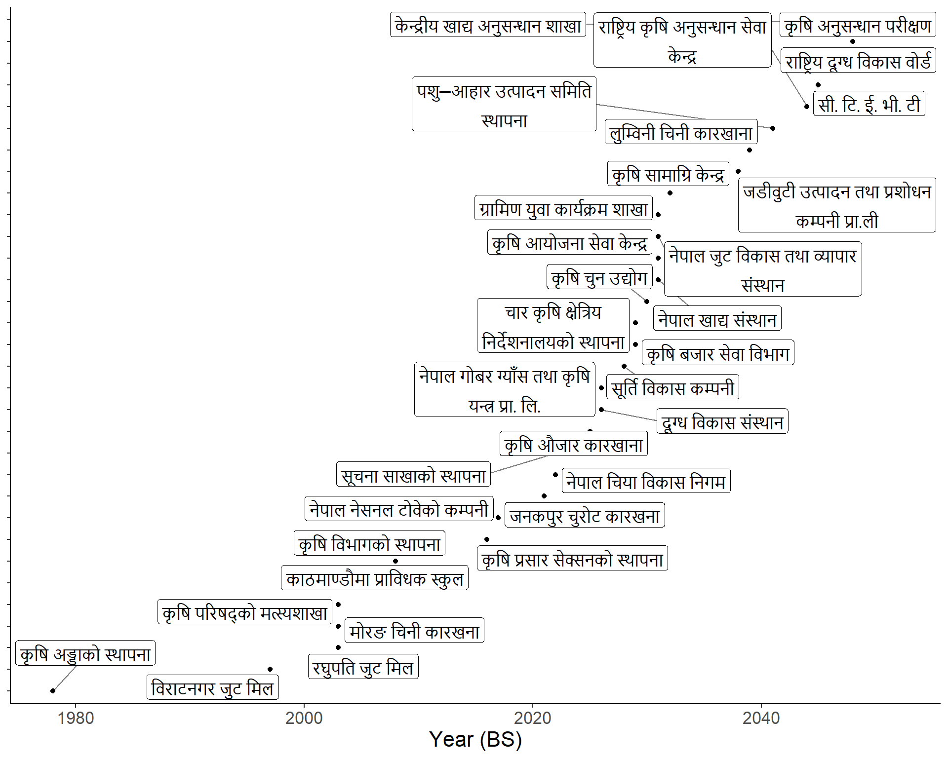
This is really a brash article meant to convey exactly what title hints at. Much of the contents are translated/transliterated from “Rice Science and Technology in Nepal: A historical, socio-cultural and technical compendium”, which was published in 2017. As of now, primary authors are left uncredited, but as entries become widely accepted, original writers and publishers will be duely recognized.

Split plot design

Design and fieldbook template

In a field experiment to test for effects of fungicide on crop, treatment of fungicides may be distinguised into multiple factors – based on chemical constituent, based on formulation, based on the mode of spray, etc. In a general case scenario where two former factors could be controlled, factor combinations may be organized in several different ways. When fully crossed implementation is not possible, split plot design comes to the rescue.

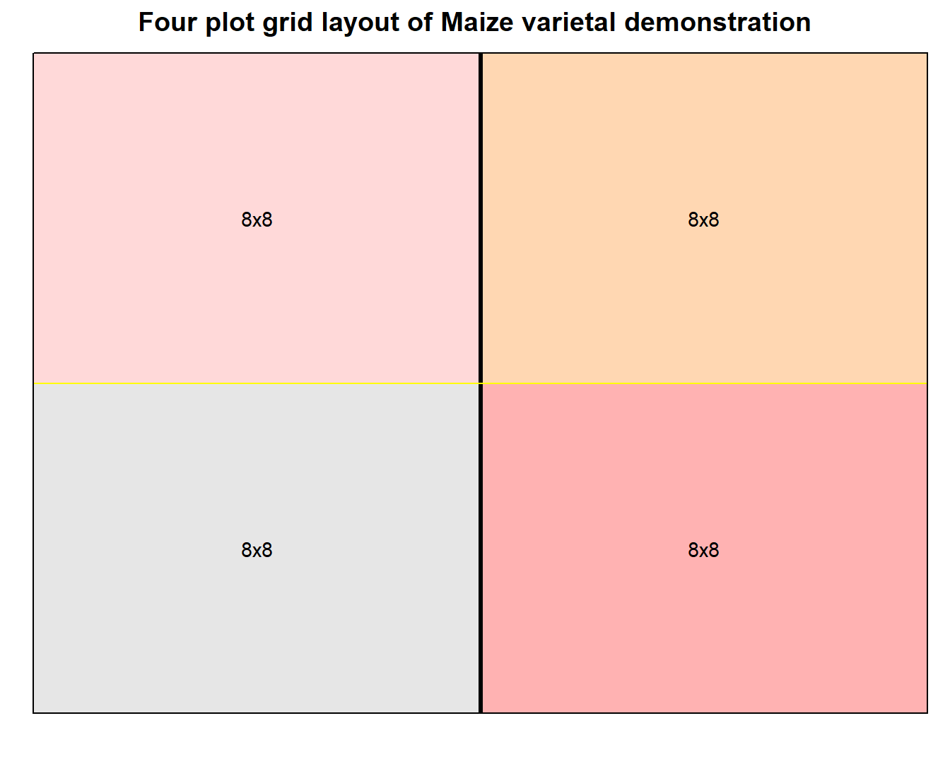
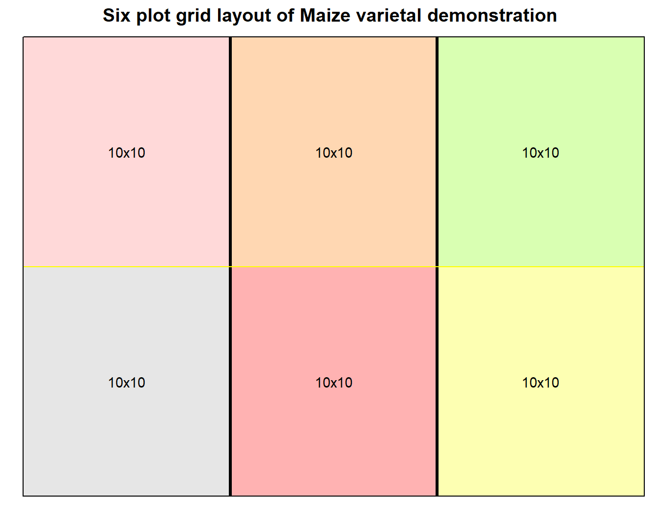
Functional approach to creating and combing multiple plots

This approach highlights features of gridExtra package that allows combining multiple grob plots using function calls. We explicitly use lapply/split or similar class of purrr functions to really scale the graphics.

We load a Hybrid maize trial dataset, with fieldbook generated using agricolae::design.rcbd(). The dataset looks as shown in Table 1, after type conversion and cleaning.

For the given dataset, we can draw on the information that Rep variable was used as field level blocking factor (Although separate, Block, variable exists, it was nested inside the Rep.) Therefore, to begin with, we ignore other spatial grouping variable. Now, since the grid graphics only requires two way represenation of plotting data, we have row and col information feeding for that.

Introduction

Balanced block designs are a class of randomized experimental design that contain equal number of records for a particular level of categorical variable across all blocks.

Example 1

Let us generate some data from random process mimicking a single factor process consisting of 3 levels.

Flow diagrams are jam-packed with information. They normally describe a process and actors that are involved in making that happen.

With r package diagram, which uses r’s basic plotting capabilities, constructing flowcharts is as easy as drawing any other graphics.

This post expands on creating simple flowdiagrams using example scenario of a wheat breeding program. The information for this graph was, most notably, deduced from those provided by senior wheat breeder of Nepal, Mr. Madan Raj Bhatta.

Toolbox for working with Unicode and Nepali fonts

Here’s a collection of excellent python scripts to convert back and forth among unicode and preeti font. To convert unicode text to preeti font:

https://github.com/globalpolicy/UnicodeToPreeti

To convert preeti font to unicode text:

https://github.com/globalpolicy/PreetiToUnicode

This one is my effort to compose an updated database on the current situation of lentil germplasm in Nepal. I’ve managed to list out the varieties that have been made available so far (either through release or registration process). Although, a lot of other popular genotypes are trending in cultivation as of now. I consider NARC’s varietal catalogs to be the most authentic, so have borrowed most of the information from these published documents.

Design and layout plan

Figure 1: Grid layout design of varietal demonstration for small number of plots

Dhangadhi of Kailali, Nepal remains relatively hotter during summer season with respect to average condition of terai agro-ecology. A regime of high day temperature with bright sunshine and cool night temperature along with plenty of seasonal rain during larger part of rice growing season favors good growth of rice crop in the region.

Based on a range of cultivation sowings carried out in the summer/rainy season of 2018, flowering dates were recorded for each plot of varieties, and the duration since planting to flowering was determined. Here, flowering time is ascribed to the period when approximately 50% of the anthers in each plots could be promptly seen as extruding. I summarize the resulting days to flowering period in the bar chart shown in Figure 1.

Mating designs

Introduction

Mating designs allow for partitioning of phenotypic effects – as due to genotype, environment or interacting effects among genes and alleles. Using one or more of these mating schemes, identification of heterotic groups, estimation of general and specific combining abilities and testing of environmental interactions could be done. Progenies resulting from a well designed mating are used for the dissection of trait genetics.

Meaning of stability

Comparison of treatments may also imply cross comparison of their stability across multiple environments, especially when a study constitutes a series of trials that are each conducted at different locations and/or at different periods in time (henceforth referred to as MET; Multi-Environment Trial). Several situations exist where only mean based performance analysis are regarded inconclusive.

For example, in varietal release process the authorizing body seeks record of consistent trait performace of certain crop genotype. The imperative is: a variety needs to be stably exhibit it’s characters in the proposed domain of cultivation, which generally is a wide area, throughout a long duration of cultivation cycles. This pre-condition of stable character inheritance is more relevant to crops constituting a homogenous and homozygous population. Either of the location, time period or combination of both, more commonly framed as year in field researches, could be assumed to present an unique environment that treatment entries are tested in. Thus, for results to be widely applicable, performance measures across environments should be more or less stable. To the contrary, the concept of utilizing differential character expression across different environments is often explored when interaction between genotypes and environments result in more desirable character.

library(lpSolve)
library(tidyverse)

Issue

A farmer has 600 katthas of land under his authority. Each of his katthas of land will either be sown with Rice or with Maize during the current season. Each kattha planted with Maize will yield Rs 1000, requires 2 workers and 20 kg of fertilizer. Each kattha planted with Rice will yield Rs 2000, requires 4 workers and 25 kg of fertilizers. There are currently 1200 workers and 11000 kg of fertilizer available.